Excel Tricks with Tejraj

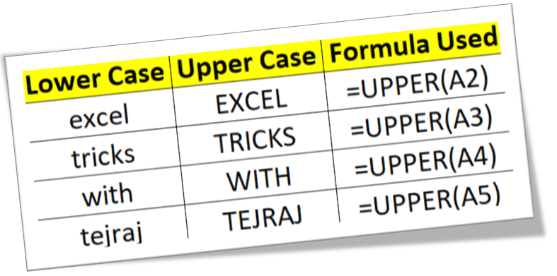
In this blog post we will learn to convert text from lower case to upper case. To convert text from lower case to upper case, we will use “UPPER” function in excel. We will learn this with the help of dummy data as shown in below image. In 1st column we have some text which is in lowercase. In 2nd column, we will use excel function which will help to convert the text from 1st column (which is in lower case) into upper case. We have to select the cell in which we want the output in “upper case” (In this case we have selected the 1st cell from 2nd column). Now, type the formula “=UPPER(A2)” in selected cell (Here “A1” is the cell address of 1st cell from 1st column). After writing the formula, we have to just hit “enter” button on our keyboard. With this we can see the text in now converted in to Upper Case in selected cell. To convert the text from lower case to upper case in remaining cells, we have to just copy and paste the above formula. In below image you can see the formula which

In this blog post we will learn to Insert Multiple Rows in excel based on cell value with the help of VBA Code. For this we have prepared dummy data as shown in below image. In this data we have listed few “Products”, their “Quantities” and their “Unit Price”. Now we want to insert multiple rows based on their “Quantities”. For example, “Product 1” has 04 quantities so we have to add 04 rows below the Product 1, “Product 2” has 02 quantities so we have to add 02 rows below the Product 2 and so on. To avoid wasting our time by manually inserting rows one by one, we can use VBA code which will do our work within seconds. To do this, just follow the below steps: 1. Add “Developer Tab” on the Ribbon if it is not already added. If you are not aware about how to add Developer Tab on the Ribbon then click here . Once added on the Ribbon, “Developer Tab” will looks like as highlighted with red in below image. 2. Now, click on the “Visual Basic” command as highlighted in below image. 3. Once

In this blog post we will learn to protect the workbook structure in excel. First of all let’s understand what it means by protecting workbook structure. Once we protect the workbook structure: 1. User cannot insert new worksheet . 2. User cannot delete existing worksheet. 3. User cannot rename worksheet . 4. User cannot hide & unhide the worksheet . 5. User cannot change the tab color . 6. User cannot copy the existing worksheet . 7. User cannot move the existing worksheet . Now, we will see how to protect worksheet structure in excel: 1. Click on “File” option on Ribbon. 2. Click on “Info” option as highlighted in below image. 3. Click on “Protect Workbook” option as highlighted in below image. 4. It will appear further options under “Protect Workbook”. Out of these options we have to click on “Protect Workbook Structure”. 5. Once we click on “Protect Workbook Structure” option, one dialog box will appear on our excel screen as shown in below image. Under this we have to check th

In this blog post we will learn to restrict the cells to accept only “Time” with the help of “Data Validation” functionality in excel. For example, we want to ask user to enter the Time in a cell but the condition is that the entered Time should be between “Start Time” and “End Time”. If user enters any other Time beyond this range then the highlighted cell should not accept it. For this we will use “Data Validation” functionality in excel. “Data Validation” can be found in “Data” tab under “Data Tools” group. Now let’s see how we can use this “Data Validation” command to restrict cell to accept only “Time”: 1. Select the cells in which we wish to restrict the “time”. In this case we want to restrict “time” in cell “B5”. 2. Click on Data Validation command under “Data Tools” group which will appear 03 further options and out of these 03 options again select “Data Validation”. 3. Once we click on “Data Validation” command, one dialog box named as “Data Validation” will appear on screen.