Excel Tricks with Tejraj

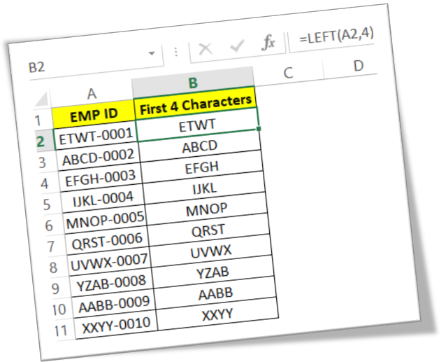
In this blog post we will learn about LEFT function in excel. With the help of this function we can extract number of characters from the beginning of the text string. Where to find LEFT function on Excel Screen: LEFT function can be found under “Text Function” category under “Formula Tab” as shown in below image: Once we click on “Text” category, we can see list of various Text Functions available in excel. LEFT function is highlighted in red in below image. Once we click on LEFT option as highlighted above, we will get the function argument dialog box as shown in below image: Syntax of LEFT Function: The Syntax of LEFT function is as below: =LEFT(text,[num_chars]) Arguments of LEFT Function: To use the LEFT function we have to use 02 arguments: Text : This is mandatory argument. We have to select the text from which we have to extract the number of characters from the beginning of the text string. Num_chars : In this argument, we have to specify the number of characters which we want

In this blog post we will learn about RIGHT function in excel. With the help of this function we can extract number of characters from the end the of the text string. Where to find RIGHT function on Excel Screen: RIGHT function can be found under “Text Function” category under “Formula Tab” as shown in below image: Once we click on “Text” category, we can see list of various Text Functions available in excel. RIGHT function is highlighted in red in below image. Once we click on RIGHT option as highlighted above, we will get the function argument dialog box as shown in below image: Syntax of RIGHT Function: The Syntax of RIGHT function is as below: =RIGHT(text,[num_chars]) Arguments of RIGHT Function: To use the RIGHT function we have to use 02 arguments: Text : This is mandatory argument. We have to select the text from which we have to extract the number of characters from the end of the text string. Num_chars : In this argument, we have to specify the number of characters which we wa

In this blog post, we will learn to convert text in “Proper Case” in excel. What is Proper Case? Proper case is somewhat different than “lower case” and “upper case”. In lower case all the letters are in “lower case” whereas in upper case all the letters are in “upper case”. But in Proper Case, first word from each word is in “upper case” and all the other letters are in “lower case”. Converting Text in Proper Case: Now we will learn to convert the text into Proper Case with simple example. For this we prepared dummy data as shown in below image. In the first column we have inserted input text which we will convert into Proper Case in the next Column. For this we will use “PROPER” function which is readily available in excel. First of all select the cell in which we have to convert the input text in Proper Case. In this case we have selected cell “B2”. Now, type “=PROPER(A2)” in cell “B2”. Once we type above function in cell “B2”, we have to just hit enter button on our keyboard. This

In this blog post we will learn to convert text from upper case to lower case. To convert text from upper case to lower case, we will use “LOWER” function in excel. We will learn this with the help of dummy data as shown in below image. In 1st column we have some text which is in uppercase. In 2nd column, we will use excel function which will help to convert the text from 1st column (which is in UPPER case) into lower case. We have to select the cell in which we want the output in “lower case” (In this case we have selected the 1st cell from 2nd column). Now, type the formula “=LOWER(A2)” in selected cell (Here “A2” is the cell address of 2nd cell from 1st column). After writing the formula, we have to just hit “enter” button on our keyboard. With this we can see the text is now converted in to lower case in selected cell. To convert the text from upper case to lower case in remaining cells, we have to just copy and paste the above formula. In below image you can see the formula which