Excel Tricks with Tejraj

In this blog post we will learn to about PI function in excel. PI function will return value of Pi which is mathematical constant which has value of 3.14. The PI function in excel return the value of Pi accurate to 15 digits. Importance of PI Function? Pi can be used to solve many mathematical problems. So if you are thinking to solve some mathematical problems for example to “calculate area of circle” or to “calculate the circumference of circle” (these are just few examples) then you can use the PI function effectively. Where to find PI function on Excel Screen: PI function can be found under “Math & Trig” function category under “Formulas” tab and under “Function Library” group as shown in below image: Once we click on “Math & Trig” function category, we can see list of various Math & Trig functions available in excel. PI function is highlighted in blue in below image. Once we click on PI option as highlighted above, we will get the function argument dialog box as shown ...

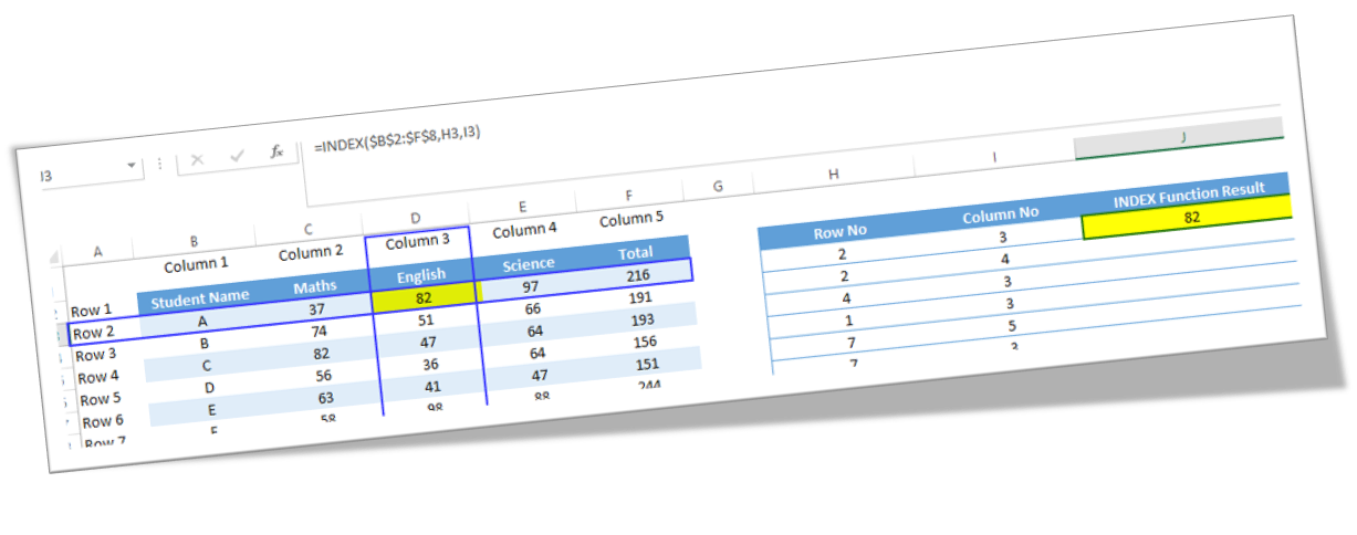
In this blog post we will learn to about INDEX function in excel. We can use INDEX function to find value which is present at the intersection of provided row number and column number in g given cell range . For example, we want to find our which value is present at the intersection point of row 3 and column 4 in a given table then applying INDEX function is a perfect solution. Where to find INDEX function on Excel Screen: INDEX function can be found under “Lookup & Reference” function category under “Formulas” tab and under “Function Library” group as shown in below image: Once we click on “Lookup & Reference” function category, we can see list of various Lookup & Reference functions available in excel. INDEX function is highlighted in blue in below image. Once we click on INDEX option as highlighted above, we will get the select argument dialog box as shown in below image. As this function has multiple argument lists, we must select one of the two argument lists appearing...

In this blog post we will learn to about MATCH function in excel. We can use MATCH function to find relative position of a provided item in a cell range . For example, we have listed name of few countries in one column, and we want to find out the relative position of specific country in that cell range then we can do so by using MATCH function. Where to find MATCH function on Excel Screen: MATCH function can be found under “Lookup & Reference” function category under “Formulas” tab and under “Function Library” group as shown in below image: Once we click on “Lookup & Reference” function category, we can see list of various Lookup & Reference functions available in excel. MATCH function is highlighted in blue in below image. Once we click on MATCH option as highlighted above, we will get the function argument dialog box as shown in below image: Syntax of MATCH Function: The Syntax of MATCH function is as below: =MATCH(lookup_value, lookup_array, [match_type]) Arguments of ...

In this blog post we will learn to about CHOOSE function in excel. CHOOSE function will choose a value or an action to perform based on the provided index number. Where to find CHOOSE function on Excel Screen: CHOOSE function can be found under “Lookup & Reference” function category under “Formulas” tab and under “Function Library” group as shown in below image: Once we click on “Lookup & Reference” function category, we can see list of various Lookup & Reference functions available in excel. CHOOSE function is highlighted in blue in below image. Once we click on CHOOSE option as highlighted above, we will get the function argument dialog box as shown in below image: Syntax of CHOOSE Function: The Syntax of CHOOSE function is as below: =CHOOSE(index_num, value1, [value2], …) Arguments of CHOOSE Function: CHOOSE function have below arguments. index_num : This argument decides which value argument is to be selected. We must provide number between 1 to 254. If we are providing...

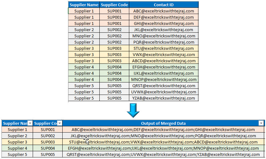
In this blogpost, we will learn to merge data from duplicate rows into a single cell in excel. Many times, we may face a situation where we have duplicate entries in rows,  and we want to merge the data from these duplicate entries into single cell. This post is perfect solution for similar problems. Let us understand this solution with simple example. Let us assume that we have a supplier database in which we have multiple contacts listed for same supplier in multiple rows (as shown in below image). In this database, Supplier 1 with unique supplier code has 03 different Contact IDs listed in 03 different rows and same scenario is with Supplier 2, Supplier 3, Supplier 4 and Supplier 5. Now we want to merge these multiple Contacts IDs for respective supplier in a single cell separated by semicolon (;). To merge data from multiple rows into a single cell in excel, follow below simple steps: Before following the below steps make sure “Supplier Code” column is sorted (Sort Type is...