Excel Tricks with Tejraj

In this blog post we will learn to “Insert Picture in Excel”. With this we can insert the images which are stored on our computer. For this you have to just follow below listed easy steps. 1. Select the cell where you want to insert picture. We have selected cell “A1” as shown in below image. The cell address of this selected cell we can see in Name Box . 2. Once we select the cell , go to Insert tab on the Ribbon where we will find command “Picture” under Illustrations group. 3. Once we click on this “Picture” command, one dialog box named as “Insert Picture” will appear on our excel screen as shown in below image. 4. Click on the picture which we want to insert in excel. Here we have clicked on the picture which is logo of our blog Excel Tricks with Tejraj . Once we click on the desired picture, name of selected picture will automatically reflect in “File Name” field (as highlighted with red box in below image). 5. After this, click on “Insert” button. 6. Once we click on this ...

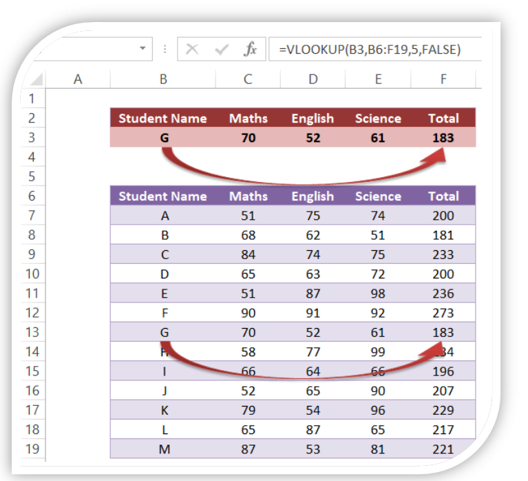
In this blog post we will see how we can apply VLOOKUP in excel. For this we have prepared a dummy data as shown in the below image. This data is divided into two groups. Blue Highlighted Data : This data contains Student Names and marks obtained by each student in the subject Maths, English and Science. In the last column we have calculated total marks obtained by each student. Red Highlighted Data : This data contains similar headers as that of Blue Highlighted data. We will apply VLOOKUP in these cells. Methods to find VLOOKUP Function on Excel Screen: We can find VLOOKUP function using two different methods. In this first method , VLOOKUP function can be found in “Lookup & Reference” which we can find in “Function Library” group under “Formulas” tab (Below screenshot for your reference). Once we click on this “VLOOKUP”, one dialog box named as “Function Arguments” will appear on excel screen. There are total 04 arguments available for this VLOOKUP function. Once we enter all th...

In this blog post we will learn to apply filter on “ Font Colors ” in excel. For this we have a data of some electronic products sold in East, West, South and North regions from 1st Aug 2019 to 1st Apr 2021 with us and we have applied font colors to this data. We have applied two font colors “Red” and “Blue” to some values under column “No of Items Sold”. We will now see how we can apply filters on Font Colors in above data: 1. Select the entire data on which we wish to apply filter on font colors. 2. Go to “Data” tab and click on the “Filter” command (Data tab and Filter command are highlighted with red in below image). 3. Once we click on the “Filter” command, we can see that drop down button is now applied to all the cells in header row as shown in red highlighted area. 4. Click on the drop down button for cell “No of Items Sold” from header row. This will show us further options to apply the filter for values in this entire column. 5. Now, select the option “Filter by Color” as h...

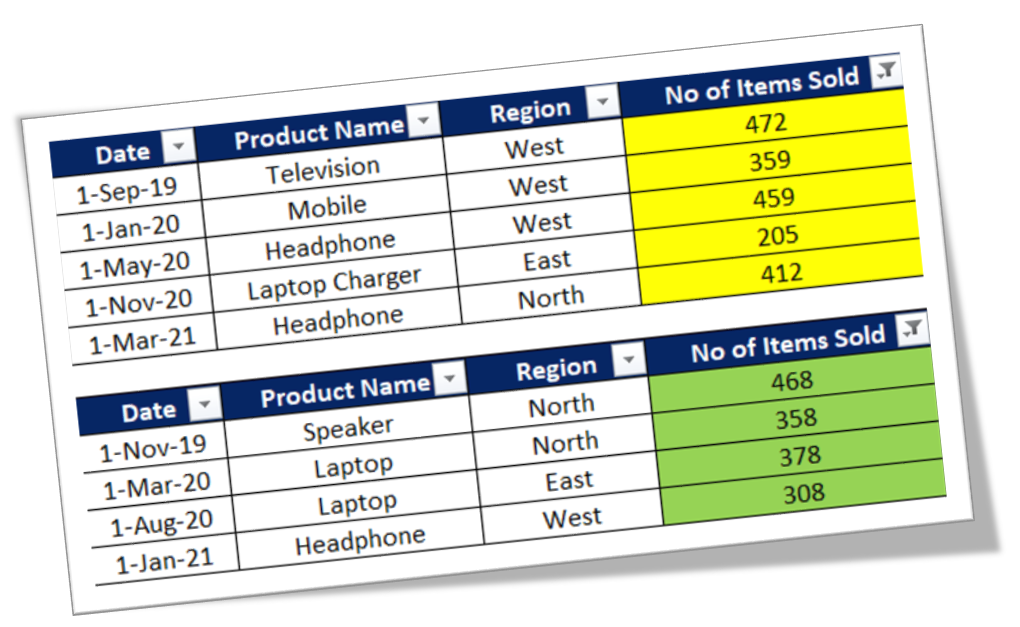
In this blog post we will learn to apply filter on “Cell Colors” in excel. For this we have a data of some electronic products sold in East, West, South and North regions from 1st Aug 2019 to 1st Apr 2021 with us and we have applied colors to this data. We have applied two colors “Yellow” and “Green” to some values under column “No of Items Sold”. We will now see how we can apply filters on cell colors in above data: 1. Select the entire data. 2. Go to “Data” tab and click on the “Filter” command (Filter command is highlighted with red in below image). 3. Once we click on the “Filter” command, we can see that drop down button is now applied to all the cells in header row. 4. Click on the drop down button for cell “No of Items Sold”. This will appear further options to apply the filter for values in this entire column. 5. Now, select the option “Filter by Color”. 6. Once we click on this option, we can see further options to apply filter by all the cell colors which we have applied in t...