Excel Tricks with Tejraj

Merge command is used to combine adjacent cells.   Unmerge command is used to separate out each cells from combined cells. How to Merge Cells? 1. Select the adjacent cells which we want to merge. 2. Go to “Alignment” group which is available under the “Home” Tab and click “Merge & Center” command. 3. Selected cells will be merged into single cell. How to Unmerge the Cells? 1. Select cells which are already merged. 2. Go to “Alignment” group which is available “Home” Tab and click “Merge and Centre” command. 3. Selected merged cells will now be separated out into multiple cells. Multiple Merge options available in Excel: 1. Merge and Center 2. Merge Across 3. Merge Cells 4. Unmerge Cells We will see what is the difference between all these? We have selected 25 cells as shown in below image. We will see the different outputs by selecting all the above listed options. 1. Merge and Cent

If we want to highlight the values which are present between two given values then we can use Conditional Formatting. YouTube Video For example we have a database of 05 students for marks obtained by them in three subjects Maths, English and Science. Now we want to highlight the marks which are between "65" to "85". To do so we can use Conditional Formatting. Let us see detailed explanation as below: 1. Select all the cells from which we want to highlight the marks. 2. Go to Home Tab. Select "Conditional Formatting", then select “Highlight Cells Rules”, then select “Between” option from the list of appeared list. 3. Now, you will see “Between Window” on your screen. Enter 1st value and 2nd value between which we want to highlight the values. Also select the formatting style from the list of list of appeared style. Below is the image for your reference. 4. We have entered 1st value as “65” and 2nd value as “85” as

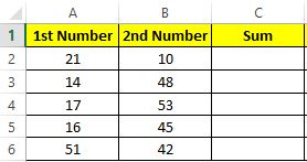
When we are working with formulas or functions in excel we have to deal with Absolute or Relative Reference or combination of these two in Excel. These reference styles are basically associated with cell address of the cells where we are using any formulas or function.  We will see these reference style one by one.  In excel “Relative Reference” style is a default reference style. Relative Reference: To explain “Relative Reference” we will use formula to calculate sum of two numbers. In “Column A” we have listed 1st number and in “Column B” we have listed 2nd number. To add the number listed in “Column A” and “Column B” we have used a formula in “Column C” as shown in below image. The output of this formula is also shown beside. Now, copy the formula from cell “C2” to the cells C3, C4, C5 and C6. The output of addition will be seen as shown in below image. Now select Range “C2:C6” where we have copied the formula to add the numbers from cell “C1”. Selec

Many times we need to Hide or Unhide rows while working in excel. So in this blog post we will see how to Hide or Unhide rows in excel. To do so, we have entered a text “Row 1” in first row of excel, “Row 2” in second row of excel and so on till “Row 5” in fifth row of excel. We have also highlighted these rows with various colors just for easy identification.  First we will see how to Hide rows and then see how we can unhide them. How to Hide Rows: 1. Select the rows which we want to hide (In this case we have selected “Row 2” and “Row 3”). 2. Go to Home Tab. Click on Format Command under Cells Group. Select “Hide & Unhide” option from list of appeared options. Again select “Hide Rows” option. 3. You can see “Row 2” and “Row 3” are now hidden.    Alternate Method to Hide Rows: 1. Select the rows which we want to hide (In this case we have selected “Row 2” and “Row 3”). 2. Press Mouse Right Click button and

Many times we need to Hide or Unhide Columns while working in excel. So in this blog post we will see how to Hide or Unhide columns in excel. To do so, we have entered a text “Column A” in first column of excel, “Column B” in second column of excel and so on till “Column E” in fifth column of excel. We have also highlighted these columns with various colors just for easy identification.  First we will see how to Hide columns and then see how we can unhide them. How to Hide Columns: 1. Select the columns which we want to hide (In this case we have selected “Column B” and “Column C”). 2. Go to Home Tab. Click on Format Command under Cells Group. Select “Hide & Unhide” option from list of appeared options. Again select “Hide columns” option. 3. You can see both the columns “Column B” and “Column C” are now hidden. Alternate Method to Hide Columns: 1. Select the columns which we want to hide (In this case we have selected “Column B”