Excel Tricks with Tejraj

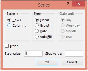
In our previous post " Fill Series in Excel " we have seen all the details about " Fill Series " options. Let us see the examples of each option in this blog post. Fill Series: Linear Trend In this section we will see how we can fill series with linear trend using fill series. Suppose, we want to fill series 1, 2, 3…. upto 20 in a column.  1. Enter value 1 in any cell and select this cell. Go to “Home Tab” then select “Editing Group” then select “Fill Command” then select “Series option” and Input the values as mentioned below in Series Dialog Box:      a. Series in: Column      b. Type: Linear      c. Step Value: 1      d. Stop Value: 20 2. Once you click on “OK” button then you will see a desired series on your screen. Fill Series: Growth Trend In this section we will see how we can fill series with Growth Trend using fill series. Suppose, we want to fill series for which the series pattern will be like: 2, 4, 8…. upto 2000 in a column. 1. Enter value 2 in any cel

In our previous post “ Fill Up, Down, Right & Left in Excel ”, we have seen fill up, fill down, fill right and fill left commands in excel. Now, in this post we will see “Fill Series” command in excel. The basic difference between “ fill up, fill down, fill right and fill left commands ” and “Fill Series” command in excel is that: “fill up, fill down, fill right and fill left commands” fills the data as it is. It is similar to copy the data from one cell to selected cells. But “Fill Series” command help us to fill the data in series. It means it helps us to fill the data in certain pattern. Also we can customize the series in which we want to fill the data with the help of options available in this command. Select “Home Tab” then select “Editing Group” then select “Fill Command” (Image is given below for your reference) Once we click on “Fill” command, various fill options will display on our screen. Select “Series” option from it. Once we click on “Series” option then we will ge

Excel has many great tricks which can help us to save our time while working on big data. In this blog post we are going to see one of those tricks where we can fill the data to the upwards of the selected cells, to the downwards of the selected cells, to the right of the selected cells and to the left of the selected cells. There are many situations where we may need to copy the data from selected cell to the upward, downward, left and right cells. But how can we do so?? In excel we can do so with the help of “Fill” command. This command we can found in: Home Tab --> Editing Group --> Fill Command. Let’s take an example. We have inserted a text “Tejraj” in a cell “D5”. Now we will see how to fill this text from cell D5 to Up, Down, Right & Left. Fill Down: 1. Let’s assume that we have to fill the data from cells D5 to D10. For this, select the Cell Range D5:D10. Keep in mind that the data from 1st cell of the selected Cell Range will fill down in entire selection. 2. Select

In our last blog post we have seen how we can create Pivot Table in Excel . If you have not yet aware of how to create Pivot Table in Excel you can click here and then continue reading this post. Let’s assume we are creating Pivot Table for data as shown in below image. Slicers are very effective while creating dashboards in excel. We can say that Slicers are “Pictorial Filters”. While we are creating Pivot Table, we are getting 04 Pivot Table areas as shown in below image. Slicers are related to “Filters” area.  Let’s create Pivot Table to summarize regional sales data. 1. Drag “Region” field into “Rows” area 2. Drag “Total Sales INR” field into “Values” area 3. Drag “Year” field into “Filters” area. This will create Pivot Table into as shown in below image. One important thing to note here is that filter is now created for field ‘”Year”. If we want to change our summary for any specific year then we can select respective year in that filter.  For example,  If want to see the su

Pivot Table in excel is a very powerful feature which helps us to to organize and summarize the data in very effective manner, that too without using any complex excel formula or functions. In this blog post we will see how to create Pivot Table in Excel. Below is the dummy sales data for last three years (2018, 2019 & 2020). In this sales data employees A, B, C & D sales various electronic components like Resistor, Capacitor, Inductor, Diodes & LED in all South, East, North & West region of India. Creating Pivot Table: Now we will see how to create Pivot Table in Excel. Pivot Table feature is available in Insert Tab. Pivot Table command is available in "Insert Tab" under "Tables Group" as shown in below image. Once you click on Pivot Table command, “Create Pivot Table” dialog box will appear on screen. This is like as shown in below image. This “Create Pivot Table” dialog box is very important to create Pivot Table. There are two important options a