Excel Tricks with Tejraj

Data Sorting is an excellent feature available in excel. With this feature we can sort the data which will provide easy data readability. In this post we will see 04 types of Data Sorting in excel. 1. A to Z Sorting 2. Z to A Sorting 3. Sort Smallest to Largest 4. Sort Largest to Smallest Let’s take an example. We have a data listed of marks obtained by few students in Maths, Science and English. Now we will apply all the four types of data sorting which we have mentioned above one by one. A to Z Sorting: A to Z sorting can be applied on cells which have alphabetic characters in them. So in our case we can apply this type of sorting only on column “Student”. 1. Select any cell from the available data. Go to “Data” tab then “Sort & Filter” group and then you have to select “Sort” command. 2. Now “Sort” dialog box will open as shown in below image. Enter the values as below: Column : Student Sort On : Values Order : A to Z 3. We can see that the values listed under “Student” column

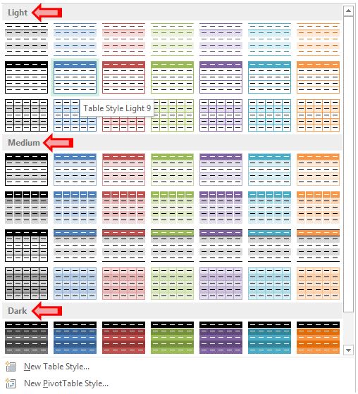
By using “Table Format” functionality in Excel we can convert our data into beautiful and attractive formats. Converting data into “Table Format” will gives us many advantages over normal data range. We will start this post by seeing how to convert data into “Table Format”.                                              Let’s take an example of sales done by 05 employees in Q1, Q2, Q3 and Q4 as shown in below image. We will use this data to convert it into “Table Format”. Just follow below steps: 1. Select any cell from the available data. In our case we have selected cell from top left corner of the data. 2. Go to “Home” Tab. 3. Select “Format as Table” command in Styles group. 4. Once you click on “Format as Table” command, various table styles will appear on screen. These table styles are divided in 03 categories Light, Medium and Dark. Select any of these Table Style. 5. “Format As Table” window will appear on our screen as shown in below image. Click OK. 6. Once we click OK then we

In previous posts on Conditional Formatting, we have seen how we can: 1. Highlight Values Greater Than Given Value 2. Highlight Values Less Than Given Value 3. Highlight Values Between Two Given Values 4. Highlight Duplicate Values In this post we will see how we can highlight values which are equal to the provided value. YouTube Video We have created dummy data of sales of 05 employees in 04 quarters Q1, Q2, Q3 and Q4. Now as an example we will see how we can highlight the cells in which sales is exactly equal to 500. To do so, follow the below steps: 1. Select the cells from which we want to highlight the cells which are equal to 500. 2. Now, go to Home Tab, then select Conditional Formatting, then select Highlight Cells Rules and then select “Equals To” option. 3. You will see “Equal To” Dialog Box appeared on your screen. 4. As we want to highlight the cells which are exactly equal to the value of 500, we have to enter value “500”

If you are following my Blog regularly then till this time you are familiar with: 1. Cell is an intersection of Rows and Columns .  2. Rows are denoted by numbers like 1, 2, 3…. till last row 16,48,576. 3. Columns are denoted by capital letters like A, B, C… till last column XFD. Considering above three points, we can find out the cell address of any cell from our excel sheet. As we know, Cell Address is denoted by column number followed by row number in double inverted comma. i.e. cell address of cell which is situated in 3rd column and 3rd row is written as “C3”. This cell address we can also see in " Name Box " as shown in below image. But there might be some scenarios where we came across situations where: 1. Columns are denoted by numbers (1, 2, 3…) instead of Capital Letters (A, B, C…). 2. Cell address is not shown in the format which is shown in above image (i.e. Cell address for cell situated in 3rd column and 3rd row is not written as “C3”). Basi