Excel Tricks with Tejraj

Have you ever tried highlighting cells from your excel worksheet which contains specific text? You might have tried this method manually. It means you might have searched the specific text which you want to highlight in entire worksheet and then you might have applied specific color of your own choice to all those cells which has the specific text. But this manual process is very tedious and time consuming. You have to search each and every entry with specific text and then highlight each valid entry. If you were working on a huge data then it may take hours to complete this task manually. Conditional Formatting is an excellent feature available in excel. With the help of Conditional Formatting we can highlight cells which contains the specific text within seconds. Let us take an example with real time data. We have listed marks of 10 students with grades obtained by them. If you want to highlight the cells manually which are having Grades “B” then you have to check each entry one by o...

Pictorial visualization speaks more effectively in data representation. Keeping this in mind in this post we are going to see how we can create “Column Charts in Excel”. Converting data into Column charts will help us to analyze the data quickly. To explain in a very simple way, we have listed salary received by 05 persons. Person A is having salary of Rs. 15000, Person B is having salary of Rs. 13000, Person C is having salary of Rs. 17000, Person D is having salary of Rs. 18000 and Person A is having salary of Rs. 20000. Now we have to convert this data into Column Chart. This is so easy. Just follow below steps: 1. Select the data which we want to convert into Column Chart. 2. Go to Insert Tab, Select "Insert Columns Chart" command under “Charts” group. 3. You will get a window which displays various options of Column Chart. Select “Clustered Column” option under “2-D Column” as shown in below image. 4. You will see "Column Chart...

Data Sorting is an excellent feature available in excel. With this feature we can sort the data which will provide easy data readability. In this post we will see 04 types of Data Sorting in excel. 1. A to Z Sorting 2. Z to A Sorting 3. Sort Smallest to Largest 4. Sort Largest to Smallest Let’s take an example. We have a data listed of marks obtained by few students in Maths, Science and English. Now we will apply all the four types of data sorting which we have mentioned above one by one. A to Z Sorting: A to Z sorting can be applied on cells which have alphabetic characters in them. So in our case we can apply this type of sorting only on column “Student”. 1. Select any cell from the available data. Go to “Data” tab then “Sort & Filter” group and then you have to select “Sort” command. 2. Now “Sort” dialog box will open as shown in below image. Enter the values as below: Column : Student Sort On : Values Order : A to Z 3. We can see that the values listed under “Student” column...

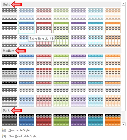
By using “Table Format” functionality in Excel we can convert our data into beautiful and attractive formats. Converting data into “Table Format” will gives us many advantages over normal data range. We will start this post by seeing how to convert data into “Table Format”.                                              Let’s take an example of sales done by 05 employees in Q1, Q2, Q3 and Q4 as shown in below image. We will use this data to convert it into “Table Format”. Just follow below steps: 1. Select any cell from the available data. In our case we have selected cell from top left corner of the data. 2. Go to “Home” Tab. 3. Select “Format as Table” command in Styles group. 4. Once you click on “Format as Table” command, various table styles will appear on screen. These table styles are divided in 03 categories Light, Med...