Merge data from Duplicate Rows into a Single Cell in Excel.
In this blogpost, we will learn to merge data from duplicate rows into a single cell in excel. Many times, we may face a situation where we have duplicate entries in rows, and we want to merge the data from these duplicate entries into single cell. This post is perfect solution for similar problems. Let us understand this solution with simple example.
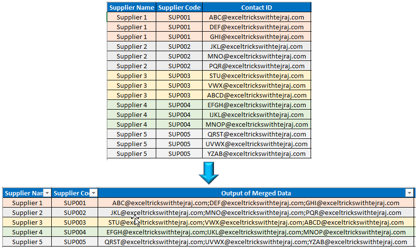
Let us assume that we have a supplier database in which we have multiple contacts listed for same supplier in multiple rows (as shown in below image).
In this database, Supplier 1 with unique supplier code has 03 different Contact IDs listed in 03 different rows and same scenario is with Supplier 2, Supplier 3, Supplier 4 and Supplier 5.
Now we want to merge these multiple Contacts IDs for respective supplier in a single cell separated by semicolon (;).
To merge data from multiple rows into a single cell in excel, follow below simple steps:
Before following the below steps make sure “Supplier Code” column is sorted (Sort Type is A to Z) if this column is not already sorted. In this case this column is already sorted from A to Z.
1. Add one helper column in above data where we will merge multiple contact IDs. In this case we have added helper column in “Column D” and named this column as “Output of Merged Data”.
2. Select cell D2 where we will enter one formula with the help of which we can merge the contact IDs for duplicate supplier names or duplicate supplier codes.
The formula we will enter is: =IF(B2=B1,CONCATENATE(D1,";",C2),C2)
3. Once we hit “Enter” button, we can see the result of this formula. But keep in mind that this is not our final result.
4. Copy this formula and paste it in the remaining cells in column D. With this we can see the result of this formula in all the remaining cells as well.
5. Now we have to remove duplicate entries and keep only one entry in which multiple Contact IDs got merged. For this we will add another helper column in “Column E” to count how many times each supplier is duplicated.
6. Select cell E2 in which we will enter a formula which will count how many times each supplier is duplicated based on Supplier Code.
The formula we will enter is: =COUNTIF($B2:$B$16,B2)
7. Once we press “Enter” button on our keyboard then we will see the result in cell E2 as shown in below image.
9. Now we have to apply filter in column E, and we will filter only values “1” from this column as shown in below image.
10. Once we press “OK” button highlighted in yellow in above image, we will see the result as shown in below image.
11. Now we have to just hide “Column C” by selecting any cell from column C and press “Ctrl” and “0” keys together on our keyboard. (To learn more about hiding columns in excel click here).
12. Similarly hide “Column E” as well and the appeared result will be our final result.
In this way, we can merge data from duplicate rows in single cell.


Comments
Post a Comment