INDEX Function in Excel
In this blog post we will learn to about INDEX function in excel.
Once we click on “Lookup & Reference” function category, we can see list of various Lookup & Reference functions available in excel. INDEX function is highlighted in blue in below image.
Once we click on OK button in above dialog box, we will get function arguments dialog box as shown in below image.
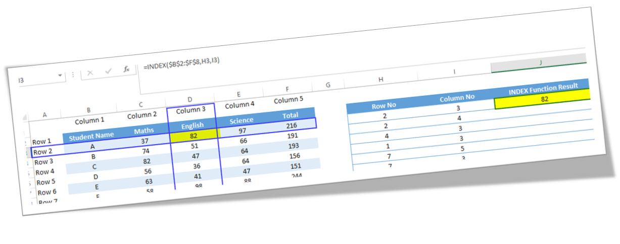
From this data, if we want to find out the value which is at the intersection of provided row number and provided column number then INDEX function is the best solution for this. We will find the values from various rows and columns as per the combination provided in below table with the help of INDEX function.
We can use INDEX function to find value which is present at the intersection of provided row number and column number in g given cell range.
For example, we want to find our which value is present at the intersection point of row 3 and column 4 in a given table then applying INDEX function is a perfect solution.
Where to find INDEX function on Excel Screen:
INDEX function can be found under “Lookup & Reference” function category under “Formulas” tab and under “Function Library” group as shown in below image:
Once we click on INDEX option as highlighted above, we will get the select argument dialog box as shown in below image. As this function has multiple argument lists, we must select one of the two argument lists appearing in this dialog box. In this case, we have selected 1st list.
Syntax of INDEX Function:
The Syntax of INDEX function is as below:
=INDEX(array, row_num, [column_num])
Arguments of INDEX Function:
INDEX function takes below arguments.
array: We have to select cell range in this argument.
row_num: We need to provide row number from selected cell range in this argument.
[column_num]: We need to provide column number from selected cell range in this argument.
Important Note:
The row number and column number we are talking above is not a row and column number of excel sheet. We are talking about the row number and column number of a selected cell range or array from 1st argument.
Below image will help you to understand this.
Example of INDEX Function:
Let’s learn to use INDEX function with the below example. We have listed names of few students and marks obtained by them in various subjects as shown in below image.
Now we will apply INDEX function to find out our desired result. For this select a cell where we want to apply INDEX function.
Apply INDEX function in selected cell as shown in below image.
Once we press enter button on our keyboard then we can see the output of INDEX function.
To find the output in remaining cells just copy and paste the INDEX function in remaining cells. We see the output as shown in below image.
In this way we can use INDEX function in excel.


Comments
Post a Comment