CHOOSE Function in Excel

Where to find CHOOSE function on Excel Screen:
CHOOSE function can be found under “Lookup & Reference” function category under “Formulas” tab and under “Function Library” group as shown in below image:

Once we click on “Lookup & Reference” function category, we can see list of various Lookup & Reference functions available in excel. CHOOSE function is highlighted in blue in below image.

Once we click on CHOOSE option as highlighted above, we will get the function argument dialog box as shown in below image:

Syntax of CHOOSE Function:
The Syntax of CHOOSE function is as below:
=CHOOSE(index_num, value1, [value2], …)

Arguments of CHOOSE Function:
CHOOSE function have below arguments.
index_num: This argument decides which value argument is to be selected. We must provide number between 1 to 254. If we are providing any formula or a reference to a number, then it should be between 1 to 254.
Value1: We can provide any value or formula or function or any cell reference which will get selected based on the index number as defined above.
We can provide maximum 255 value arguments from value1 to value254.
Example of CHOOSE Function:
Let’s learn to use CHOOSE function with the below example. We have prepared a dummy data as shown in below screenshot. In this data we have mentioned employee ratings and their performance based on these rating.
We will learn to use CHOOSE function with this data to check the performance of employee based on the provided rating.


In selected cell “C10”, we will apply CHOOSE function as shown in below image.

Press enter button but with this we will an error in our output. This is because we have not yet provided any index number in cell B10.


Similarly, we can select other index numbers from drop down list and the output of CHOOSE function will change accordingly.
In this way, we can use CHOOSE function in excel.


Comments
Post a Comment