Applying VLOOKUP in Excel

For this we have prepared a dummy data as shown in the below image. This data is divided into two groups.
Blue Highlighted Data: This data contains Student Names and marks obtained by each student in the subject Maths, English and Science. In the last column we have calculated total marks obtained by each student.
Red Highlighted Data: This data contains similar headers as that of Blue Highlighted data. We will apply VLOOKUP in these cells.

Methods to find VLOOKUP Function on Excel Screen:
We can find VLOOKUP function using two different methods.
In this first method, VLOOKUP function can be found in “Lookup & Reference” which we can find in “Function Library” group under “Formulas” tab (Below screenshot for your reference).

Once we click on this “VLOOKUP”, one dialog box named as “Function Arguments” will appear on excel screen. There are total 04 arguments available for this VLOOKUP function. Once we enter all the 04 arguments we can get the desired output.

In this second method, we have to press “=” button and then type “VLOOKUP” word and after that we have to type open bracket “(“. With this, all the 04 arguments will pop up on the screen. Once we enter all the 04 arguments we can get the desired output.

Arguments of VLOOKUP Function:
There are total 04 argument for VLOOKUP function as listed below:
1. Lookup Value: This is the value which we want to look. Our VLOOKUP output will be based on this value. This is mandatory argument.
2. Table Array: This is the table in which we want to look the “Lookup Value”. This is mandatory argument.
3. Column Index Number: In this argument we have to enter number of column from which we want the output. This is mandatory argument.
4. Range Lookup: This argument is optional. This argument again contains two sub-arguments TRUE or FALSE.
a. TRUE: It will find the “closest” match of Lookup value.
b. FALSE: It will find the “exact” match of Lookup value.
Now we will see how we can apply VLOOKUP to find the marks obtained by selected student in subjects Maths, English and Science as well as to find the Total marks. We have applied Drop Down List in cell “B3” where we can select the Students Name by using this Drop Down List.

In this example, we have selected Student Name “G” with the help of Drop Down List and we will apply the VLOOKUP based on this value.

To Find Marks in Maths using VLOOKUP Function:
1. Select the cell “C3”.

2. Apply the VLOOKUP function and enter all the 04 arguments as listed below:
a. Lookup Value: We want to look Student Name, hence in this argument we will select cell “B3” where we have already selected the Student Name “G”.
b. Table Array: Select all the cells from Blue Highlighted Data as we want to find the marks obtained by Student “G” from this table.
c. Column Index Number: Enter number “2” in this argument as we are calculating marks obtained in Maths and they are listed in 2nd column from the Lookup value in our table array.
d. Range Lookup: Enter FALSE in this argument as it will find the “exact” match of our Lookup value.
Below image is for your reference.
Below image is for your reference.

3. Once we enter all the 04 arguments, hit enter button on keyboard and we can see the VLOOKUP output.

To Find Marks in English using VLOOKUP Function:
1. Select the cell “D3”.

2. Apply the VLOOKUP function and enter all the 04 arguments as listed below:
a. Lookup Value: We want to look Student Name, hence in this argument we will select cell “B3” where we have already selected the Student Name “G”.
b. Table Array: Select all the cells from Blue Highlighted Data as we want to find the marks obtained by Student “G” from this table.
c. Column Index Number: Enter number “3” in this argument as we are calculating marks obtained in English and they are listed in 3rd column from the Lookup value in our table array.
d. Range Lookup: Enter FALSE in this argument as it will find the “exact” match of our Lookup value.
Below image is for your reference.

3. Once we enter all the 04 arguments, hit enter button on keyboard and we can see the VLOOKUP output.

To Find Marks in Science using VLOOKUP Function:
1. Select the cell “E3”.

2. Apply the VLOOKUP function and enter all the 04 arguments as listed below:
a. Lookup Value: We want to look Student Name, hence in this argument we will select cell “B3” where we have already selected the Student Name “G”.
b. Table Array: Select all the cells from Blue Highlighted Data as we want to find the marks obtained by Student “G” from this table.
c. Column Index Number: Enter number “4” in this argument as we are calculating marks obtained in Science and they are listed in 4th column from the Lookup value in our table array.
d. Range Lookup: Enter FALSE in this argument as it will find the “exact” match of our Lookup value.
Below image is for your reference.

3. Once we enter all the 04 arguments, hit enter button on keyboard and we can see the VLOOKUP output.

To Find Total Marks using VLOOKUP Function:
We can also calculate the Total marks obtained by Student “G” with the help of SUM function but this blog post is specifically for learning VLOOKUP, we will use VLOOKUP function to calculate total marks.
1. Select the cell “F3”.

2. Apply the VLOOKUP function and enter all the 04 arguments as listed below:
a. Lookup Value: We want to look Student Name, hence in this argument we will select cell “B3” where we have already selected the Student Name “G”.
b. Table Array: Select all the cells from Blue Highlighted Data as we want to find the marks obtained by Student “G” from this table.
c. Column Index Number: Enter number “5” in this argument as we are calculating total marks and they are listed in 5th column from the Lookup value in our table array.
d. Range Lookup: Enter FALSE in this argument as it will find the “exact” match of our Lookup value.
Below image is for your reference.

3. Once we enter all the 04 arguments, hit enter button on keyboard and we can see the VLOOKUP output.

With the above listed steps, you can easily apply VLOOKUP function in excel.


Comments
Post a Comment