Applying Filter on Icon Sets in Excel
In this blog post we will learn to apply filter on “Icons Sets” in excel.
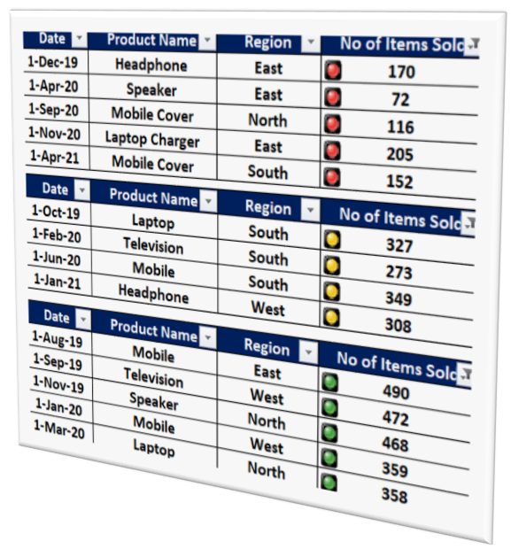
For this we have a data of some electronic products sold in East, West, South and North regions from 1st Aug 2019 to 1st Apr 2021 with us and we have applied Icon Sets to this data. We have applied 3 Traffic Light Icon Sets to values under column “No of Items Sold”.

We will now see how we can apply filters on these Icon Sets in above data:
1. Select the entire data on which we wish to apply filter on Icon Sets.


4. Click on the drop down button for cell “No of Items Sold” from header row of the data on which we have applied Icon Sets. This will show us further options to apply the filter for Icon Sets in this entire column.


7. Click on any desired Icon Set Color on which we want to apply the filter. In this case we have selected “Red Traffic Light” color and we can see that all the values with this “Red Traffic Light” Icon will get filtered as shown in below image.

8. If we select the “Green Traffic Light” in step no. 6 then we can see that all the values with this “Green Traffic Light” Icon will get filtered as shown in below image.

9. Similarly, if we select the “Yellow Traffic Light” in step no. 6 then we can see that all the values with this “Yellow Traffic Light” Icon will get filtered as shown in below image.

In this way, you can apply filter on Icon Sets in Excel.


Comments
Post a Comment