Customize SmartArt Graphic in Excel
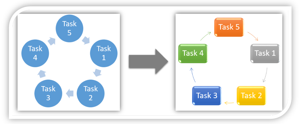
If you are not familiar about how to insert SmartArt Graphic in excel then click here before reading this blog post. We will take same example which we have taken in our previous blog post about inserting SmartArt Graphic in excel. In that blog post, we have inserted below SmartArt Graphic.

Where to find commands to Customize SmartArt Graphic on Excel Screen:
The main thing we should know is where we can find commands to customize SmartArt Graphics on our excel screen? For this we have to click on the SmartArt Graphic which we have created.
Once we click on this SmartArt Graphic, two additional tabs as listed below will get enabled on Ribbon.
1. Design Tab
2. Format Tab

We will use these two tabs to Customize SmartArt Graphic in excel.
Note: These two tabs will get enabled if and only if we select the SmartArt Graphics. Once we click anywhere outside, then these two tabs will get disabled.
Changing Colors of SmartArt Graphic:
To change the Colors of SmartArt Graphic, follow the below stpes:
1. Select the SmartArt Graphic and click on “Design Tab”. This will show us all the commands from “Design Tab”.

2. Now click on “Change Colors” commands which is highlighted in red color in below image.


4. With this we can see that the color of our SmartArt Graphic will change according to selected color.

Changing SmartArt Styles:
1. We can also change the SmartArt style with the help of “Design Tab”. We can find all these Styles under “SmartArt Styles” group.

2. We can choose the style of our own choice. In this case we have selected the style as highlighted in below image.


Changing SmartArt Layouts:
1. We can also change the SmartArt Layouts with the help of “Design Tab”. We can find all these Layouts under “SmartArt Styles” group.

2. We can choose the Layout of our own choice. In this case we have selected the Layout as highlighted in below image.


In this way we can Customize the SmartArt Graphic in Excel.


Comments
Post a Comment