Currency Format in Excel
We have seen previously in brief about how we can “Format Cell Values in Excel”. In that blog post we have learned about converting cell values in various formats but in a brief way and now we will focus on “Currency Format in Excel” in this blog post.


1. We have created a dummy data of few employees and salary earned by each employee. You can see this data as shown in below image.

2. Select the numbers which we wish to convert into “Currency Format” and click on the “Currency” option under category. This will help us to see the additional options available under “Currency Format”.

3. We can add desired Currency symbol by selecting any of the symbols from the highlighted area as shown in below image. We can see all the available currency symbols by clicking on drop down button. Here in this example we have selected currency symbol as “$ English (Australia)”.


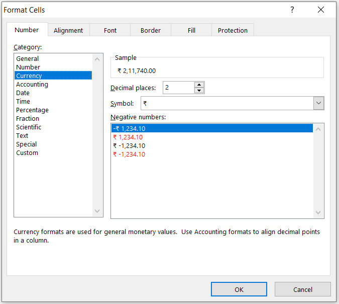
c. Third option will same as first option which will highlight negative numbers in black color with negative sign in currency format.

d. Last option will highlight negative numbers in red color with negative sign in currency format.

I hope you can now use the "Currency Format" in excel wisely in your daily excel work.
In our previous blog post we have seen different 03 methods to go to additional options of formatting cell values. If you missed to read those methods, please click here before going for this blog post.
We can use any of these 03 methods to get the “Format Cells” dialog box and select “Currency” Category as shown in below image. With this we can see all the additional options under Currency Formats in excel.
The additional options which are available under “Currency Format” are as below:

Sample: This option is common in all the formats which we can see under Category in above image which we can use to see how the selected numbers will look in currency format.
Decimal Places: With this we can increase or decrease the decimal places of selected numbers in our data in Currency Format.
Symbol: This option will add desired currency symbol to selected numbers.
Negative Numbers: This option will highlight the negative numbers in different ways in our currency format.
Decimal Places:
With this we can increase or decrease the decimal places of selected numbers in our data in Currency Format.
1. We have created a dummy data of few employees and salary earned by each employee. You can see this data as shown in below image.

2. Select the numbers which we wish to convert into “Currency Format” and click on the “Currency” option under category. This will help us to see the additional options available under “Currency Format”.

3. We can increase or decrease the decimal places of selected numbers in Currency Format by clicking on the buttons in the highlighted area in below image.

4. Once we click on “OK” button, we will see that our selected numbers will get converted into currency format with 02 decimal places.

Symbol:
This option will add desired currency symbol in front of the selected numbers.
1. We have created a dummy data of few employees and salary earned by each employee. You can see this data as shown in below image.


4. Once we click on “OK” button we can see that the selected currency symbol is now added in front of the selected numbers.

Negative Numbers:
This option will highlight the negative numbers in different ways in our currency format.
1. We have created a dummy data of profit/loss for a firm in each month as shown in below image.

2. Select the numbers from which we wish to highlight the negative numbers from currency format. Go to the “Format Cell” dialog box and select “Currency” option under category. This will display additional options from currency format to highlight the negative numbers as highlighted in below image.

3. There are total 04 different options available to display negative numbers under currency format. These options are shown in below image.

a. First option will highlight negative numbers in black color with negative sign in currency format.

b. Second option will highlight negative numbers in red color in currency format.


I hope you can now use the "Currency Format" in excel wisely in your daily excel work.


Comments
Post a Comment