Area Chart in Excel


Now we will see how we can convert this data into “Area Chart” for better data visualization.
Just follow below steps:
1. Select the above data which we want to convert into Area Chart.


Changing Chart Style:
To change the formatting of our Area Chart, click on the existing “Area Chart” and this will appear two additional tabs on our Ribbon. These tabs are:
1. Design Tab
2. Format Tab


Similarly we can select any of the Chart Style from available options as per our own choice to give special effect to our Area chart.
Changing Color of Area Chart:
If we want to change the color of above created “Area Chart” then we have to select the existing “Area Chart” and then click on “Design” tab and then click on “Change Colors” option.


Now, our “Area Chart” with “Color 3” and “Style 3” will look like as shown in below image:

Similarly we can try various Chart Styles and Color options to make our Area Chart beautiful.


Great job for publishing such a nice article. Your article isn’t only useful but it is additionally really informative. Thank you because you have been willing to share information with us. Hire Excel Expert
ReplyDeleteThank you..!!
DeleteYou have worked nicely with your insights that make our work easy. The information you have provided is really factual and significant for us. Keep sharing these types of articles, Thank you.Excel Consultant
ReplyDeleteGlad to hear that you found the information provided in this blog post useful. Thank you for your kind words...!
Delete