XOR Function in Excel
In this blog post we will learn about “XOR” function Excel. This function is categorized as “Logical Function” in Excel.
XOR Function Returns “TRUE” output when "Number of TRUE Conditions" provided in expressions are odd and it returns “FALSE” when “Number of TRUE Conditions” are even.
When we click on “XOR Function” the following window will appear on screen. We can enter the logical conditions in the respective fields.


=XOR(logical1,[logical2],…)
Logical1: We can provide 1st condition in this argument. This is mandatory argument.
[Logical2]: We can provide 2nd condition in this argument. This is optional argument.
We have to provide minimum one condition to use XOR function properly but there is limit of entering maximum 254 conditions in XOR function. We cannot enter more than 254 conditions in XOR function.

In this example we can see how XOR Function Returns “TRUE” output when "Number of TRUE Conditions" provided in expressions are odd and it returns “FALSE” when “Number of TRUE Conditions” are even.

In above example:
In the 1st row the “number of TRUE conditions” are odd so the output is “TRUE”.
In the 2nd row “number of TRUE conditions” are even so the output is “FALSE”.
In the 3rd row “number of TRUE conditions” are odd so the output is “TRUE”.
In the 4th row “number of TRUE conditions” are even so the output is “FALSE”.
In the 5th row “number of TRUE conditions” are odd so the output is “TRUE”.
In the 6th row “number of TRUE conditions” are even so the output is “FALSE”.
I hope you are now clear with the concept of “XOR Function” in excel. With this you can now use “XOR Function” in your daily excel work whenever required.
XOR Function Returns “TRUE” output when "Number of TRUE Conditions" provided in expressions are odd and it returns “FALSE” when “Number of TRUE Conditions” are even.
How to find XOR Function on Excel Screen:
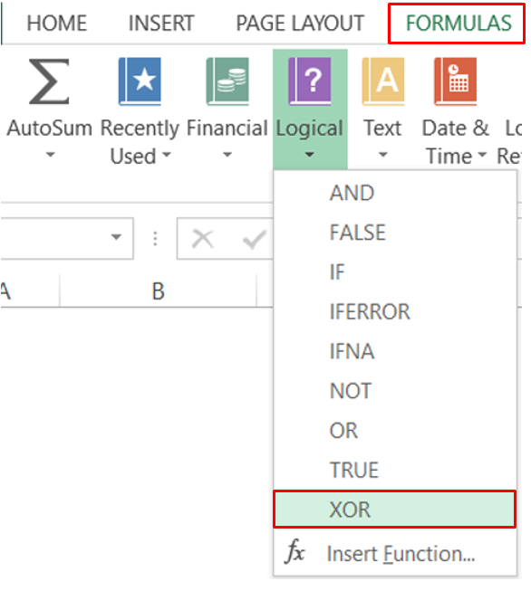
To find XOR function on our excel screen, go to “Formula Tab” & click on “Logical” command, which will appear all the Logical functions available in excel. We can see “XOR function” as highlighted in below image.

Alternatively we can also find XOR function by pressing “=” key and typing word “XOR” as shown in below image.

Syntax of XOR Function:
The syntax of XOR function is as below:=XOR(logical1,[logical2],…)
Arguments of XOR Function:
XOR function have following arguments:Logical1: We can provide 1st condition in this argument. This is mandatory argument.
[Logical2]: We can provide 2nd condition in this argument. This is optional argument.
We have to provide minimum one condition to use XOR function properly but there is limit of entering maximum 254 conditions in XOR function. We cannot enter more than 254 conditions in XOR function.

Example of XOR Function:
Now, we will see how to make use of this XOR function by taking simple example.In this example we can see how XOR Function Returns “TRUE” output when "Number of TRUE Conditions" provided in expressions are odd and it returns “FALSE” when “Number of TRUE Conditions” are even.

In the 1st row the “number of TRUE conditions” are odd so the output is “TRUE”.
In the 2nd row “number of TRUE conditions” are even so the output is “FALSE”.
In the 3rd row “number of TRUE conditions” are odd so the output is “TRUE”.
In the 4th row “number of TRUE conditions” are even so the output is “FALSE”.
In the 5th row “number of TRUE conditions” are odd so the output is “TRUE”.
In the 6th row “number of TRUE conditions” are even so the output is “FALSE”.
I hope you are now clear with the concept of “XOR Function” in excel. With this you can now use “XOR Function” in your daily excel work whenever required.


Comments
Post a Comment