Conditional Formatting: Highlighting Bottom 10 Items
This blog post is in continuation to our series of posts on “Conditional Formatting”. In this blog post we will see how to highlight Bottom 10 Items in Excel?
But, before proceeding on this topic, first we should know where we can find “Conditional Formatting” option in Excel. We can find “Conditional Formatting” in “Home” tab and under Home Tab go to “Styles” group.

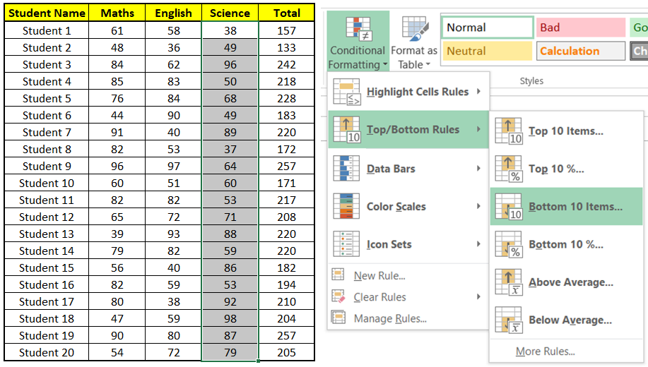
We can find many sub categories under “Conditional Formatting”. But the one which we will focus in this blog post is to highlight “Bottom 10” Items. Below image will help you to find the exact option to highlight “Bottom 10 Items”.


Now we will see how we can highlight “Bottom 10” Items in column Total i.e. we will highlight the cells which contain Bottom 10 total marks from all the students.


3. Once we click “OK” button, “Bottom 5” Items from our selection will get highlighted with selected formatting style “Yellow Fill with Dark Yellow Text”.


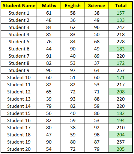
Now you are familiar with the option where we can find the option to highlight “Bottom 10” Items. To explain this topic in very simple way, I have created a dummy data of 20 students and marks obtained by them in subjects Maths, English & Science. Also we have used SUM function to calculate the total marks obtained by each student.

We will use this dummy data to highlight “Bottom 10” Items.
1. Select the cells from which we wish to highlight “Bottom 10 Items”. In our case we have selected cells from column “Total” and then selected the option “Bottom 10 Items” as shown in below image.

2. “Bottom 10 Items” dialog box will now pop up on our screen. Under this we have to provide two inputs:
1st Input: Here we have to select “10” as we wish to highlight “Bottom 10” Items.
2nd Input: Here we have to select the formatting style. In this case we have selected formatting style as “Green Fill with Dark Green Text”.
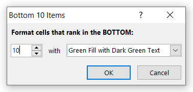
Once we click “OK” button, “Bottom 10 Items” from our selection will get highlighted with selected formatting style “Green Fill with Dark Green Text”.
Example 1: Highlighting “Bottom 5” Items:
In this example we will see how we can highlight “Bottom 5” Items from the selected cells.
1. Select the cells from which we wish to highlight “Bottom 5” Items. In our case we have selected cells from column “Maths” and then selected the option “Bottom 10” Items as shown in below image.

2. “Bottom 10 Items” dialog box will now pop up on our screen. Under this we have to provide two inputs:
1st Input: Here we have to select “5” as we wish to highlight “Bottom 5” Items.
2nd Input: Here we have to select the formatting style. In this case we have selected formatting style as “Yellow Fill with Dark Yellow Text”.


Example 2: Highlighting “Bottom 3” Items:
1. Select the cells from which we wish to highlight “Bottom 3” Items. In our case we have selected cells from column “Science” and then selected the option “Bottom 10” Items as shown in below image.

2. “Bottom 10 Items” dialog box will now pop up on our screen. Under this we have to provide two inputs:
1st Input: Here we have to select “3” as we wish to highlight “Bottom 3” Items.
2nd Input: Here we have to select the formatting style. In this case we have selected formatting style as “Light Red Fill with Dark Red Text”.

3. Once we click “OK” button, “Bottom 3” Items from our selection will get highlighted with selected formatting style “Light Red Fill with Dark Red Text”.

With this we can highlight Bottom “N” values where you can replace value of “N” with positive integers as per your wish so that you can highlight Bottom “N” Items.


Comments
Post a Comment