Data Bars in Conditional Formatting
In continuation to series of posts on Conditional Formatting, we will learn how to use Data Bars in Conditional Formatting through this post.


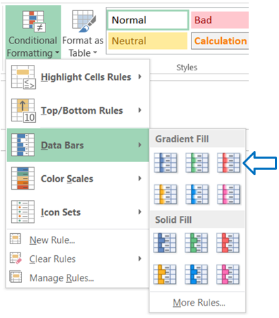
2. All the “Data Bars” colors will now appear on our screen. Out of these we have to go to "Gradient Fill" and then select “Red Data Bars”.


Conditional Formatting command can be found in Styles group under Home tab as shown in below image.

Click on the Conditional Formatting option and select “Data Bars” option from the list of appeared options. We can now see all the “Data Bar” options available in excel.
These “Data Bar” options are categorized into two groups.
1. Solid Fill
2. Gradient Fill:
There are six different “Data Bar” colors available in each group. These colors are listed below:
1. Blue Data Bar
2. Green Data Bar
3. Red Data Bar
4. Orange Data Bar
5. Light Blue Data Bar
6. Purple Data Bar
Each group with their respective colors are shown in below image:
Solid Fill:

Gradient Fill:

Now we will see how we can apply these “Data Bars” on our data. For this we have created dummy data of few employees and Incentive received by them.

Example with Gradient Fill:
1. Select all the cells where we wish to apply “Data Bars”. (Here we have selected entire column of Incentive). Then we have to click on option “Data Bars” from “Conditional Formatting”.

3. As a result, “Data Bars” will get added on the selected cells.

Example with Solid Fill:
1. Select all the cells where we wish to apply “Data Bars”. (Here we have selected entire column of Incentive). Then we have to click on option “Data Bars” from “Conditional Formatting”.

2. All the “Data Bars” colors will now appear on our screen. Out of these we have to go to "Solid Fill" and then select “Red Data Bars”.'

3. As a result, “Data Bars” will get added on the selected cells.

Points To Remember:
1. Length of “Data Bars” will depend on the values available in selected cells.
2. Excel automatically detects the maximum and minimum values from selected cells and accordingly it will adjust the length of “Data Bars”
3. Higher the value longer the Bar.
4. Minimum value will get shortest Bar.
Try using “Data Bars” from Conditional Formatting and share your experiences in comment section.


Comments
Post a Comment