Find and Select Commands in Excel
In this blog post we will see all the options available under “Find & Select” command in excel.
 To explain all the options in details we have prepared a dummy data of Sales Performance for the year 2020. In this data we have entered data of few employees as shown in below image. We have applied some formulas, Data Validation, Comments, Conditional Formatting to this data so that it will be easier for you to understand this topic.


 3. This will open “Find and Replace” dialog box on our screen.


3. Go To dialog box will appear on our screen.

4. We have to provide the Cell Address of a cell where we want to jump from our current location. This cell address we have to enter under “Reference” field as shown in below image. As an example we have provided cell address of cell “B8”.

5. Click on "OK" button and as a result we can see that the cell with provided cell address i.e. “B8” is now selected.


3. As a result we can see that all the cells which are constants will get selected.


3. Now select the area from which we have to select all the objects. If we want to select all the objects from selected sheet then just press “Ctrl + A”. In our example we have only one object which is selected as shown in below image.


This command is available in Home tab, under Editing group as shown in below image.


So, let’s see all these options one by one:
Find:
This option will help us to find desired value in our existing data.
1. Select the sheet where our existing data is present.

2. Select the command “Find & Select” and select option “Find” from the list of available options.

3. This will open “Find and Replace” dialog box on our screen.

4. We have to provide input value for the field “Find what” which we have to find in our existing data. As an example we will enter value “ETWT003” in this field.

5. As a result we can see that the value “ETWT003” is selected. We can also see the cell address of this value in Name Box as well as the content on the selected cell in Formula Bar.

Replace:
This option will help us to replace the old value with new value in our existing data
1. Select the sheet where our existing data is present.

2. Select the command “Find & Select” and select option “Replace” from the list of available options.


4. In this dialog box we have to provide 02 input values:
a. Find what: This is old value which we want to replace.
b. Replace with: This is new value which will appear in our result instead of old value.
As an example we have provided the values as shown in below image.

5. Click on “Replace All” button and we can see that the old values are now replaced with new values.

Go To:
This option will help us to jump from one cell address to another cell address without using scrollbars.
1. Select the sheet where we have our existing data.

2. Select the command “Find & Select” and select option “Go To” from the list of available options.


Go To Special:
This option will help us to jump from one cell address to another cell address that too by using some special conditions.
1. Select the sheet where we have our existing data.

2. Select the command “Find & Select” and select option “Go To Special” from the list of available options.

3. This will open “Go To Special” dialog box. We will cover all these options available under this dialog box in separate blog post. Stay tuned…!!!

Formulas:
This option will help us to select all the cells which contains formula.
1. Select the sheet where we have our existing data.

2. Select the command “Find & Select” and select option “Formulas” from the list of available options.

3. As a result we can see that all the cells which contains formula will get selected.

Comments:
This option will help us to select all the cells which contains Comments.
1. Select the sheet where we have our existing data.

2. Select the command “Find & Select” and select option “Comments” from the list of available options.

3. As a result we can see that all the cells which contains Comments will get selected.

Conditional Formatting:
This option will help us to select all the cells for which Conditional Formatting is applied.
1. Select the sheet where we have our existing data.

2. Select the command “Find & Select” and select option “Conditional Formatting” from the list of available options.

3. As a result we can see that all the cells for which Conditional Formatting is applied will get selected.

Constants:
This will help us to select all the cells which are constants (Constants cells are those cells for which no any formula is applied).
1. Select the sheet where we have our existing data.

2. Select the command “Find & Select” and select option “Constants” from the list of available options.


Data Validation:
This option will help us to select all the cells for which Data Validation is applied.
1. Select the sheet where we have our existing data.

2. Select the command “Find & Select” and select option “Data Validation” from the list of available options.

3. As a result all the cells for which Data Validation is applied will get selected.

Select Objects:
This option will help us to select all the objects present in the excel worksheet.
1. Select the sheet where we have our existing data.

2. Select the command “Find & Select” and select option “Select Objects” from the list of available options.


Selection Pane:
This option will help us to open Selection Pane which is used to make the object visible or to hide them.
1. Select the sheet where we have our existing data.

2. Select the command “Find & Select” and select option “Selection Pane” from the list of available options.

3. As a result, we can see that “Selection Pane” will get open on right side of the excel screen. All the objects available on our active sheet will get listed in this section. We can hide or unhide these objects as per our requirements.

This is all about the “Find & Select” commands in excel. If you have any questions or queries, you can write in the comments box below.


Comments
Post a Comment